A bearing is a machine element that supports another moving machine element known as a journal. It enables a relative motion between the contact surfaces of the members while carrying the load. While doing so a certain amount of power is wasted in overcoming frictional resistance due to the relative motion between the contact surfaces. We need to study the types of Bearings, design, and materials used for bearings briefly. In the previous article, we discussed the different types of Bearings. Hydrodynamic Lubricated Bearings are a type of bearing that comes under Sliding Contact Bearings. In this article, let us discuss the Heat Generated in Journal Bearing.


A little consideration will show that a certain amount of power is wasted in overcoming frictional resistance due to the relative motion between the contact surfaces. There will be rapid wear if the rubbing surfaces are in direct contact. To reduce frictional resistance and wear and sometimes to carry away the heat generated, a layer of fluid known as lubricant may be provided. The lubricant used to separate the journal and bearing is usually a mineral oil refined from petroleum, but vegetable oils, silicon oils, greases, etc., may be used.
Heat Generated in Journal Bearing
The heat generated in a bearing is due to the fluid friction and friction of the parts having relative motion. Mathematically, heat generated in bearing,
Qg = μ.W.V
units: N-m/s or J/s or watts
Where
μ = Coefficient of friction
W = Load on the bearing in N = Pressure on the bearing in N/mm2 × Projected area of the bearing in mm2 = p (l × d)
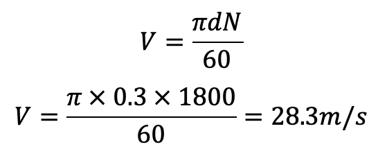
V = Rubbing velocity in m/s = (πd.N)/60 , d is in meters
N = Speed of the journal in r.p.m.
After the thermal equilibrium has been reached, heat will be dissipated at the outer surface of the bearing at the same rate at which it is generated in the oil film. The amount of heat dissipated will depend upon the temperature difference, size, and mass of the radiating surface and on the amount of air flowing around the bearing. However, for convenience in bearing design, the actual heat dissipating area may be expressed in terms of the projected area of the journal.
Heat dissipated by the bearing,
Qd = C.A (tb –ta)
Units: J/s or W
Where
C = Heat dissipation coefficient in W/m2/°C,
A = Projected area of the bearing in m2 = l × d
tb = Temperature of the bearing surface in °C
ta = Temperature of the surrounding air in °C
The value of C has been determined experimentally by O. Lasche. The values depend upon the type of bearing, its ventilation, and the temperature difference. The average values of C (in W/m2/°C), for journal bearings may be taken as follows:
For unventilated bearings (Still air) = 140 to 420 W/m2/°C
For well-ventilated bearings = 490 to 1400 W/m2/°C
It has been shown by experiments that the temperature of the bearing (tb) is approximately halfway between the temperature of the oil film (t0) and the temperature of the outside air (ta). In other words,
t b – t a = 1/2 ( t 0 – t a )
Notes :
- For a well-designed bearing, the temperature of the oil film should not be more than 60°C, otherwise, the viscosity of the oil decreases rapidly and the operation of the bearing is found to suffer. The temperature of the oil film is often called the operating temperature of the bearing.
- In case the temperature of the oil film is higher, then the bearing is cooled by circulating water through coils built into the bearing.
- The mass of the oil to remove the heat generated at the bearing may be obtained by equating the heat generated to the heat taken away by the oil. We know that the oil takes the heat away.
Qt = m.S.t
Units: J/s or watts
Where
m = Mass of the oil in kg/s
S = Specific heat of the oil. Its value may be taken as 1840 to 2100J / kg / °C
t = Difference between outlet and inlet temperature of the oil in °C.
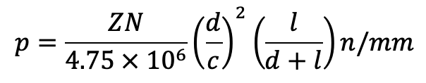
Critical Pressure of the Journal Bearing
The pressure at which the oil film breaks down so that metal-to-metal contact begins is known as critical pressure or the minimum operating pressure of the bearing. It may be obtained by the following empirical relation, i.e.
Critical pressure or minimum operating pressure,

Example problem to calculate Heat Generated in Journal Bearing
Problem Statement: The load on the journal bearing is 150 kN due to the turbine shaft of 300 mm diameter running at 1800 r.p.m. Determine the Length of the bearing if the allowable bearing pressure is 1.6 N/mm2. Amount of heat to be removed by the lubricant per minute if the bearing temperature is 60°C and viscosity of the oil at 60°C is 0.02 kg/m-s and the bearing clearance is 0.25 mm.
Answer:
Given:
W = 150kN = 150 × 103 N
d = 300 mm = 0.3 m
N = 1800 r.p.m.
p = 1.6 N/mm2
Z = 0.02 kg / m-s
c = 0.25 mm
1. Length of the bearing
Let
l = Length of the bearing in mm.
We know that the projected bearing area A = l × d = l × 300 = 300 l mm2
and allowable bearing pressure ( p),

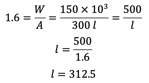
2. Amount of heat to be removed by the lubricant
We know that the coefficient of friction for the bearing,

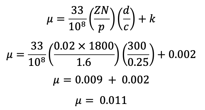
Rubbing velocity,

Amount of Heat Generated in Journal Bearing (or heat to be removed by the lubricant),
Qg = μ.W.V
Qg = 0.011 × 150 × 103 × 28.3
Qg = 46695 J/s or W
Qg = 46.695kW
A 47 kW of heat is to be removed by the lubricant for the given journal bearing.